NDF and Microfacet Model
To show what is NDF and how to derive the general formulate of Microfacet Model
Preliminary
The target of writing this post is to record my understanding of microfacet theory. It will be updated whenever my understanding is refined. I will try to derive the microfacet model in a friendly way for all the readers that want to get familiar with this theory as well. It is greatly appreciated if one can figure out the mistake in this post and show in the comment below. Also, any discussion on this topic is welcome.
Microsurface and Geometric surface
| Symbol | Definition |
|---|---|
| $\mathcal{M}$ | The surface area of microsurface |
| $\mathcal{G}$ | The surface area of geometric surface |
| $p_m$ | The point on the microsurface $\mathcal{M}$ |
| $p_g$ | The point on the geometric surface $\mathcal{G}$ |
| $\omega_g$ | The normal of the geometric surface |
| $<\cdot, \cdot>$ | The inner product of two vectors clamp to 0 |
Before get deeper into the microfacet theory, we need to answer why we need this theory. The reason is easy to realize. Let’s look at the figure below:
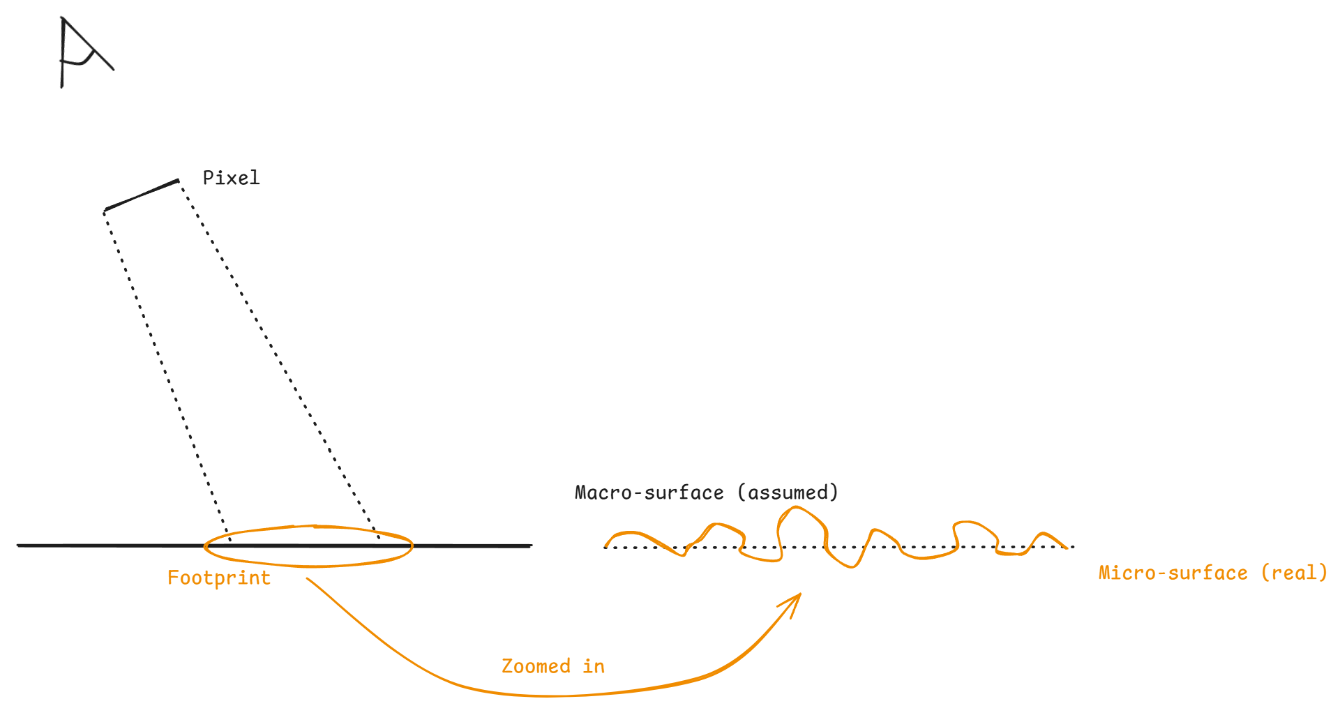
We called the area of the object surface that covered by one pixel the footprint. As illustrated in the figure, there are many complex microstructures within that footprint, we call them microsurface. Due to these microstructures, the appearance of this area should be highly spatial-varying. However, since one pixel can only return one RGB, we need to summarize the appearance of these microstructures with only one RGB value. Obviously, we need to derive the statistical (or aggregated) properities of the microsurface from its spatial properities. Once we have its statistical properites, we can assume that the area within the footprint is flat, which can use only one normal vector to describe it. called geometric surface or macrosurface. This assumed macrosurface needs a complex microfacet theory that summarizes the appearance into one value from its statistical properties. That’s why we need the microfacet model.
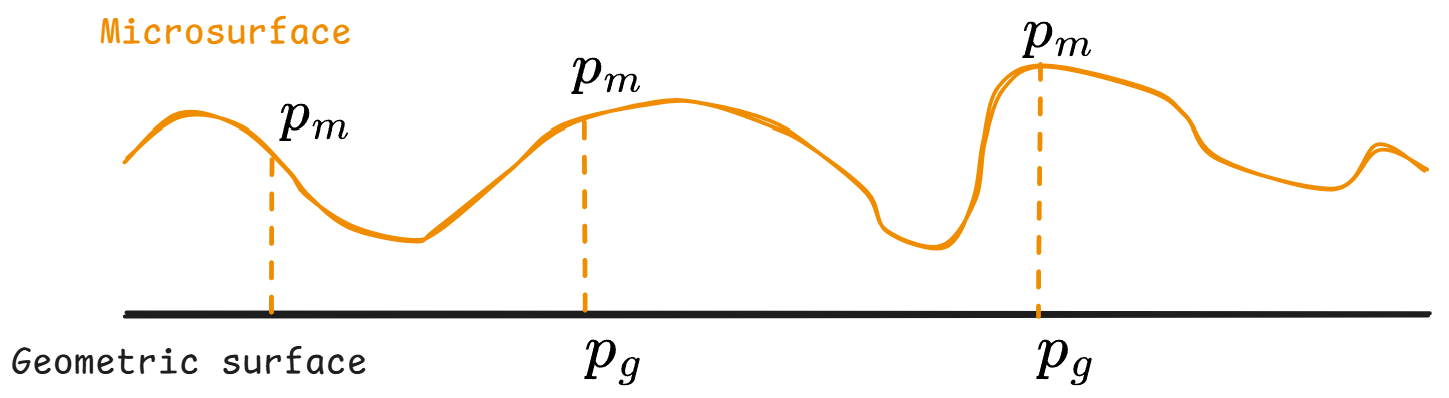
The classical microfacet theory has a basic assumption, that is there need to be a bijection between microsurface $\mathcal{M}$ and geometric surface $\mathcal{G}$.
Assumption 1: One, and only one point $p_m$ on the $\mathcal{M}$ can be projected to one point $p_g$ on the $\mathcal{G}$ along the geometric normal $\omega_g$.
This assumption leads to:
\begin{equation} \label{eq: Relationship between micro and geo} \int_{\mathcal{M}} <\omega_m(p_m), \omega_g> \mathrm{d} p_m = \int_{\mathcal{G}} \mathrm{d} p_g = A_g, \end{equation}
where $A_g$ is the area of geometric surface. One can make $A_g = 1m^2$ without loss of generality. This term will always be cancelled out in the following derivation.
Normal Distribution Function
| Symbol | Definition |
|---|---|
| $\Omega$ | The spherical space |
| $D(\omega)$ | The normal distribution function |
| $\delta_{\omega^{\prime}}(\omega)$ | The dirac delta function, $+\infty$ if $\omega = \omega^{\prime}$ and 0 otherwise, normalized in the integral |
| $\omega_i$ | The incident direction |
| $\omega_o$ | The outgoing direction |
| $\omega_m$ | The normal of one point on the \mathcal{M} |
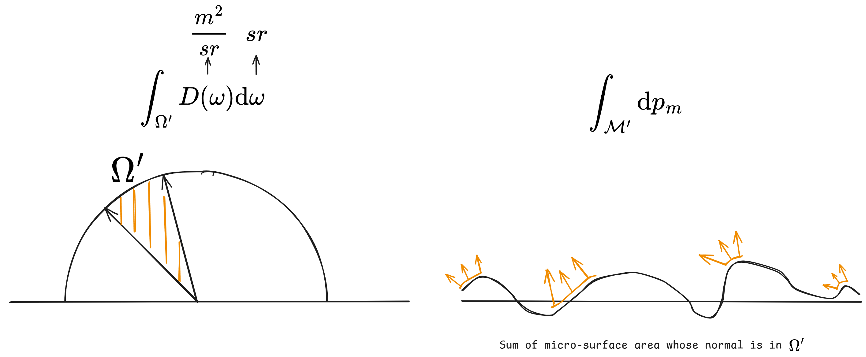
One important information we need to use to describe the microsurface’s geometric appearance, is the summary of the normal on the microsurface. We can use a function called Normal Distribution Function (NDF) to describe it. One need to distinguish it from the Probability Density Function (PDF) of normal, which describe the probability of normal of a uniformly random-sampled point on the microsurface. The definition of the NDF is:
\begin{equation} \label{eq: def of NDF} D(\omega) = \int_{\mathcal{M}} \delta_{\omega}(\omega_m(p_m)) \mathrm{d} p_m. \end{equation}
It describes the total area of the microsurface that their normal pointing at direction $\omega$. Thus, the unit of $D(\omega)$ is $\frac{m^2}{sr}$. Why we need to define the NDF? The reason is that, NDF is a bridge to connect two different spaces: one is the spatial space, that is, the microsurface space $\mathcal{M}$, and another is the statistical space, that is, the spherical space $\Omega$. An informal understanding from the relationship of unit is that, $D(\omega)\mathrm{d}\omega$ ($\frac{m^2}{sr} \cdot sr$) indicates all the differential area $\mathrm{d}p_m$ ($m^2$) whose normal pointing toward $\omega$. A more precise description of this relationship is that, given a subset $\Omega^{\prime}$ from the $\Omega$, we can have a corresponding subset $\mathcal{M}^{\prime}$ from $\mathcal{M}$ that $\mathcal{M}^{\prime}$ contains all the points on the microsurface whose normal inside the $\Omega^{\prime}$, and we have:
We need to understand the NDF well before we get into the following content, this is the base of the microfacet theory. Here are some deduction related to NDF:
Statistical area counting. The counting of the microsurface area can be converted from spatial integral to statistical integral via NDF, leading to:
\[\int_{\Omega} D(\omega) <\omega, \omega_g> \mathrm{d} \omega = \int_{\mathcal{M}} <\omega_m(p_m), \omega_g> \mathrm{d} p_m = \int_{\mathcal{G}} \mathrm{d} p_g = A_g \left(= 1m^2\right)\]Relationship between NDF and normal PDF. The unit of PDF of normal $p(\omega)$ is $\frac{1}{sr}$, so it is obviously that:
\[p(\omega) = \frac{D(\omega)}{\int_{\Omega} D(\omega) \mathrm{d} \omega},\]where the denominator is the total area of microsurface.
Masking Function
| Symbol | Definition |
|---|---|
| $W_m(p_m, \omega_o)$ | The projection factor at $p_m$ toward direction $\omega_o$ |
| $A_{proj}(\omega_o)$ | The view-depenent projected area of microsurface toward direction $\omega_o$. |
| $L(\omega_o)$ | The aggregated outgoing radiance across the whole microsurface toward $\omega_o$ |
| $L(p_m, \omega_o)$ | The outgoing radiance at the point on the microsurface $p_m$ toward direction $\omega_o$ |
| $G(p_m, \omega_o) \in {0, 1}$ | The spatial geometric masking term toward direction $\omega_o$ |
| $G(\omega_m, \omega_o) \in [0, 1]$ | The statistical geometric masking term describing the ratio of all the microsurface with normal $omega_m$ not being masked. |
The reason why we introduce the microfacet theory is to calculate the aggregated outgoing radiance from the microsurface covered by the pixel’s footprint. Thus, we need to first figure out two magnitudes: the view-dependent projected area and the formula of the outgoing radiance.
View-dependent Projected Area
This projected area measures the area of the microsurface that we can observe from one given view direction. To analyze the formula, we can assume that every differential area $\mathrm{d}p_m$ has a projection factor $W_m(p_m, \omega_o)$ toward the given view direction $\omega_o$. Thus, the projected area can be formulated as:
\[A_{proj}(\omega_o) = \int_{\mathcal{M}} W_m(p_m, \omega_o)\mathrm{d}p_m\]Due to the intrinsic of the microfacet assumption, the view-dependent projected area is always $<\omega_g, \omega_o>$, leading to:
\[\int_{\mathcal{M}} W_m(p_m, \omega_o)\mathrm{d}p_m = <\omega_g, \omega_o> = \cos\theta_o\]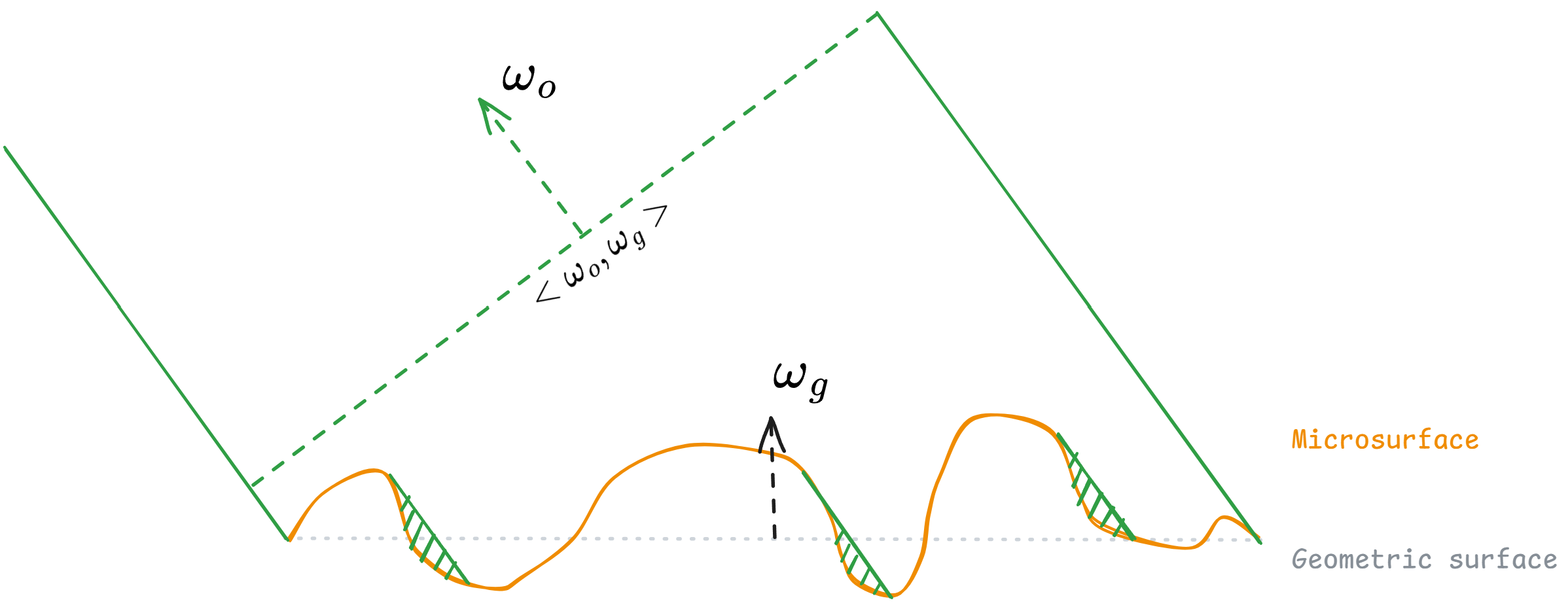
Outgoing Radiance
Obviously, observer can only receive the outgoing radiance from the view-dependent projected area, that is, the visible part of the microsurface. To formulate this, we could guess that every point $p_m$ on the microsurface should have an outgoing radiance $L(p_m, \omega_o)$ that may contribute to the final aggregated outgonig radiance $L(\omega_o)$, and the contribution weight is the view-dependent projected area of $p_m$. Since this weight is not guaranteed to be normalized, so the final formula is:
\[L(\omega_o) = \frac{\int_{\mathcal{M}} W_m(p_m, \omega_o) L(p_m, \omega_o) \mathrm{d} p_m }{\int_{\mathcal{M}} W_m(p_m, \omega_o) \mathrm{d} p_m}\]Maybe you have thought about how to convert this spatial integral into a statistical integral as before. However, we have not analyzed the components of $W_m(p_m, \omega_o)$ so far, which we will discuss in the next subsection.
Geometric Masking
Obviously, we can notice that there are many place on the microsurface whose outgoing radiance will be occluded (or masked) be another part of the microsurface. Like the visibility term, we also need to use a term called masking function $G(p_m, \omega_o)$ to indicate whether the outgoing radiance will not be occluded. After we define this masking function, the projection factor $W_m(p_m, \omega_o)$ can be represented by:
\[W_m(p_m, \omega_o) = G(p_m, \omega_o) <\omega_m(p_m), \omega_o>.\]And we can immediately get the following spatial integral equations:
\begin{equation} \label{eq: Spatial Projected Area} \int_{\mathcal{M}} G(p_m, \omega_o) <\omega_m(p_m), \omega_o>\mathrm{d}p_m = \cos\theta_o \end{equation}
\begin{equation} \label{eq: Spatial Outgoing Radiance} L(\omega_o) = \frac{\int_{\mathcal{M}} G(p_m, \omega_o) <\omega_m(p_m), \omega_o> L(p_m, \omega_o) \mathrm{d} p_m }{\int_{\mathcal{M}} G(p_m, \omega_o) <\omega_m(p_m), \omega_o> \mathrm{d} p_m} \end{equation}
Conventionally, we need to have a statistical version of the masking function. Different from the normal distribution function, the statistical masking function $G(\omega, \omega_o)$ is defined as the visible ratio of the microsurface area whose normal is pointing toward $\omega$, leading to:
\[G(\omega, \omega_o) = \frac{\int_{\mathcal{M}}\delta_{\omega}(\omega_m(p_m)) G(p_m, \omega_o)\mathrm{d}p_m}{\int_{\mathcal{M}}\delta_{\omega}(\omega_m(p_m))\mathrm{d}p_m}\]Then, the equation \eqref{eq: Spatial Projected Area} has them statistical version:
\begin{equation} \label{eq: Statistical Projected Area} \int_{\Omega} G(\omega, \omega_o) <\omega, \omega_o> D(\omega) \mathrm{d}\omega = \cos\theta_o \end{equation}
This is also a constraint of the masking function.
Microfacet BRDF
| Symbol | Definition |
|---|---|
| $f_r(\omega_i, \omega_o)$ | The microfacet BRDF |
| $f_m(p_m, \omega_i, \omega_o)$ | The microsurface BRDF at point $p_m$ |
| $f_m(\omega_m, \omega_i, \omega_o)$ | The microsurface BRDF where the normal is pointing toward $\omega_m$ |
| $G(\omega_m, \omega_i, \omega_o)$ | The shadowing-masking function |
| $R(\omega;\omega_m)$ | The pure reflected direction if the incident / outgoing direction is $\omega$ and the normal of surface is $\omega_m$. |
| $F(\omega_i, \omega_m)$ | The fresnel term. |
| $\vec{h}$ | The unnormalized half vector |
| $\omega_h$ | The normalized half vector |
To find out the formula of the microfacet BRDF $f_r(\omega_i, \omega_o)$ to satisfy:
\[\mathrm{d}L(\omega_o) = f_r(\omega_i, \omega_o) <\omega_i, \omega_g> \mathrm{d} L(\omega_i),\]we need to utilize the differential version of equation \eqref{eq: Spatial Outgoing Radiance}, which looks like:
\[\mathrm{d}L(\omega_o) = \frac{1}{\cos\theta_o} \int_{\mathcal{M}} G(p_m, \omega_o) <\omega_m(p_m), \omega_o> \mathrm{d}L(p_m, \omega_o) \mathrm{d} p_m\]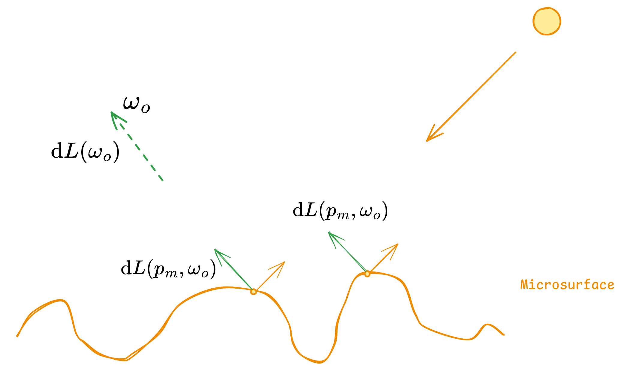
Recall that for every point on the microsurface, we have the classic rendering equation (without self-emitting):
\[L(p_m, \omega_o) = \int_\Omega f_m(p_m, \omega_i, \omega_o) L(p_m, \omega_i) <\omega_i, \omega_m(p_m)> \mathrm{d} \omega_i\]as well as the definition of the BRDF $f_m(p_m, \omega_i, \omega_o) = \frac{\mathrm{d}L(p_m, \omega_o)}{L(p_m, \omega_i) <\omega_i, \omega_m(p_m)> \mathrm{d}\omega_i}$.
Substituting the $\mathrm{d}L(p_m, \omega_o)$ term, we have:
\[\mathrm{d}L(\omega_o) = \frac{1}{\cos\theta_o} \int_{\mathcal{M}} G(p_m, \omega_i,\omega_o) f_m(p_m, \omega_i, \omega_o) L(p_m, \omega_i) <\omega_m(p_m), \omega_o> <\omega_i, \omega_m(p_m)> \mathrm{d}\omega_i \mathrm{d} p_m\]Here, we could find the the original masking function $G(p_m, \omega_o)$ has been replaced by the new shadowing-masking function. The reason is that, $p_m$ may not be directly illuminated by the light source, and this is a symmetric case to the masking-function. So we extend it into shadowing-masking function $G(p_m, \omega_i,\omega_o)$.
Since those microstructure are too tiny to have a significant difference on the location $p_m$ w.r.t. the distance between light source and geometric surface. Hence, we have a proper assumption that the incident radiance $L(p_m, \omega_i)$ is independent to the location $p_m$, leading to $L(p_m, \omega_i) = L(\omega_i)$.And the equation can be rewritten as:
\[\mathrm{d}L(\omega_o) = \frac{1}{\cos\theta_o} L(\omega_i) \mathrm{d}\omega_i \int_{\mathcal{M}} G(p_m, \omega_i,\omega_o) f_m(p_m, \omega_i, \omega_o) <\omega_m(p_m), \omega_o> <\omega_i, \omega_m(p_m)> \mathrm{d} p_m\]Comparing with the definition of $f_r(\omega_i, \omega_o)$, we have the initial formula of the microfacet BRDF:
\[f_r(\omega_i, \omega_o) = \frac{1}{<\omega_i, \omega_g><\omega_o, \omega_g>} \int_{\mathcal{M}} G(p_m, \omega_i, \omega_o) f_m(p_m, \omega_i, \omega_o) <\omega_m(p_m), \omega_o> <\omega_i, \omega_m(p_m)> \mathrm{d} p_m\]Now we obtain the spatial formula of the microfacet BRDF. To convert it into statistical integral, we need to introduce a new assumption:
Assumption 2: The material properities across all the microsurface covered by the same footprint are identical.
This assumption leads to the independency between location $p_m$ and microsurface BRDF $f_m(p_m, \omega_i, \omega_o)$, causing $f_m(p_m, \omega_i, \omega_o) = f_m(\omega_m, \omega_i, \omega_o)$. And we can have the statistical integral:
\begin{equation} \label{eq: Statistical Microfacet BRDF} f_r(\omega_i, \omega_o) = \frac{1}{<\omega_i, \omega_g><\omega_o, \omega_g>} \int_{\Omega} G(\omega_m, \omega_i, \omega_o) f_m(\omega_m, \omega_i, \omega_o) D(\omega_m) <\omega_m, \omega_o> <\omega_m, \omega_i> \mathrm{d} \omega_m \end{equation}
Hence, what we need to do next, is to show the components of microsurface BRDF $f_m(\omega_m, \omega_i, \omega_o)$.
Pure Specular BRDF
Before introducing the pure specular BRDF, let me explain why we need it. This is because of the third assumption of the microfacet theory:
Assumption 3: The microsurface is pure specular.
So what does the pure specular BRDF look like? This is what we need to solve in this subsection. To begin with, we need to first get familiar with the fresnel effect. The left image below is borrowed from Reflection, Refraction and Fresnel.
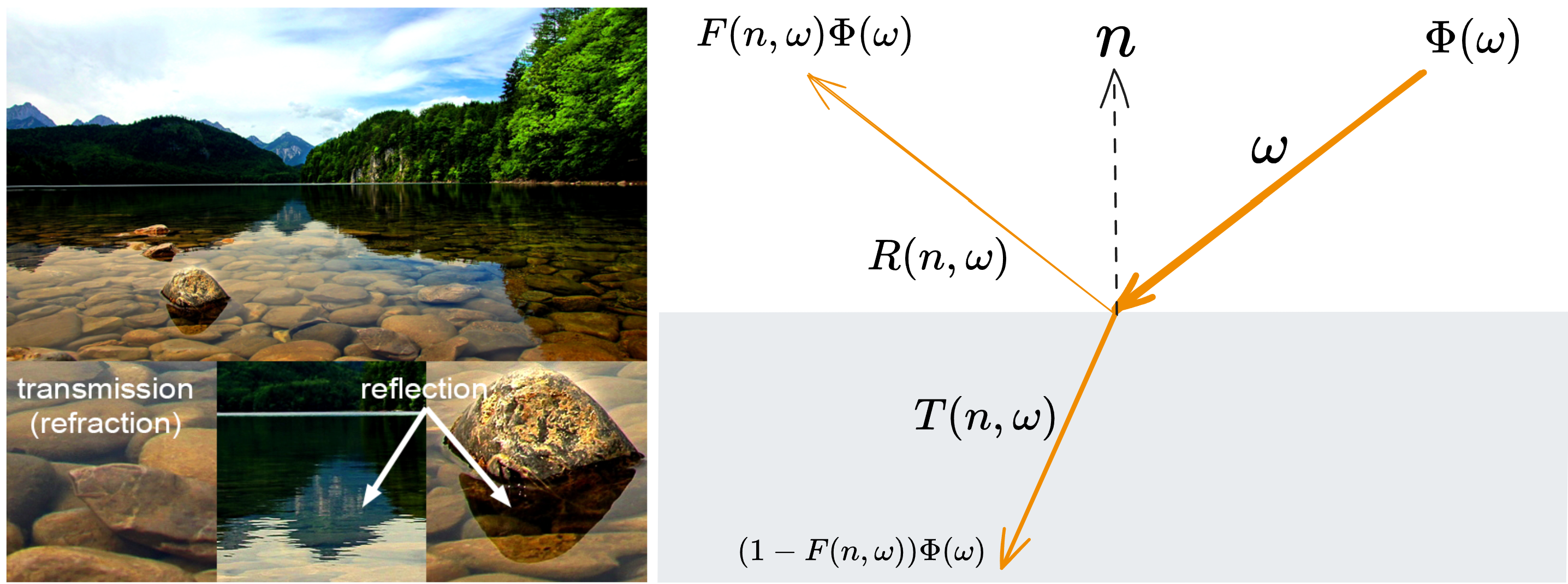
Fresnel effect describes that when the light hit on the surface, some of its energy reflected, and the order refracted. The amount of reflected energy is related to the angle of incidence. In radiosity, we need to use the energy per second, i.e., the flux, to mathematically describe this effect. Here we only consider the relationship between the reflected outgoing flux and the incident flux:
\[\mathrm{d}\Phi(\omega_o) = F(\omega_m, \omega_i)\mathrm{d}\Phi.(\omega_i)\]Since
\[\mathrm{d}\Phi(\omega)=L(\omega)\cos\theta\mathrm{d}A\mathrm{d}\omega = L(\omega)\cos\theta\mathrm{d}A\sin\theta\mathrm{d}\theta\mathrm{d}\phi,\]we have
\[L(\omega_o)\cos\theta_o\mathrm{d}A\sin\theta_o\mathrm{d}\theta\mathrm{d}\phi = F(\omega_m, \omega_i) L(\omega_i)\cos\theta_i\mathrm{d}A\sin\theta_i\mathrm{d}\theta\mathrm{d}\phi\]Due to the nature of the reflection effect, many of the terms can be cancelled out, leaving:
\[L(\omega_o) = F(\omega_m, \omega_i) L(\omega_i).\]On the other hand, since we are deriving the BRDF $f_m(\omega_m, \omega_i, \omega_o)$ of “pure specular” surface, it means that we only receive the light from the direction $\omega_i = R(\omega_o; \omega_m)$ which will reflected mirrorly to the $\omega_o$. Thus, there must be a delta term in the $f_m(\omega_m, \omega_i, \omega_o)$, leading to:
\[f_m(\omega_m, \omega_i, \omega_o) = f(\omega_m, \omega_i, \omega_o) \delta_{R(\omega_o;\omega_m)}(\omega_i).\]Subsequently, the rendering equation has become:
\begin{equation} L(\omega_o) = \int_\Omega f(\omega_m, \omega_i, \omega_o) \delta_{R(\omega_o;\omega_m)}(\omega_i) L(\omega_i) <\omega_i, \omega_m> \mathrm{d} \omega_i = f(\omega_m, R(\omega_o;\omega_m), \omega_o) L(R(\omega_o;\omega_m)) <R(\omega_o;\omega_m), \omega_m>. \end{equation}
Substituting the $L(\omega_o)$, we can get:
\[f(\omega_m, \omega_i, \omega_o) = \frac{F(\omega_m, \omega_i)}{<\omega_i, \omega_m>}.\]So, the pure specular BRDF is:
\begin{equation} \label{eq: Pure Specular BRDF} f_m(\omega_m, \omega_i, \omega_o) = \frac{F(\omega_m, \omega_i)\delta_{R(\omega_o;\omega_m)}(\omega_i)}{<\omega_i, \omega_m>} \end{equation}
Introducing Half Direction
HOWEVER, it’s too soon to celebrate; there is one more thing we need to do. Maybe you have noticed that, in the equation \eqref{eq: Statistical Microfacet BRDF}, the incident direction $\omega_i$ and the outgoing direction $\omega_o$ are fixed; the integral variable is the normal of microsurface $\omega_m$. We know that the incident radiance can reflected to the desired outgoing direction only if the normal is pointing toward the half vector between $\omega_i$ and $\omega_o$. So there is truly a delta situation. But our previous delta function is defined on the $\omega_i$ or $\omega_o$. Thus we cannot utilize it to solve the integral.
We can make the equation more concise if we can introduce the half vector $\vec{h} = \omega_i + \omega_o$ to the equation \eqref{eq: Pure Specular BRDF}. If so, one need to be very causious if the variable of the equation has changed, since the jacobian term needs to be considered. We can assume that, there are many pairs of $\omega_i$ and $\omega_o$ that have the same half vector $\vec{h}$, so the function need to have a transformation term to maintain consistency before and after replacing variable. This is called the Change of Variables Theorem.
By replacing the $\omega_o$ term (the same as $\omega_i$), we can have a new BRDF equation:
\[f_m(\omega_m, \omega_i, \omega_o) = \frac{F(\omega_m, \omega_i)\delta_{\omega_m}(\omega_h)}{<\omega_i, \omega_m>} |\frac{\partial\omega_h}{\partial\omega_o}|=\lim_{\mathrm{d}\omega_o\rightarrow0} \frac{F(\omega_m, \omega_i)\delta_{\omega_m}(\omega_h)}{<\omega_i, \omega_m>} |\frac{\mathrm{d}\omega_h}{\mathrm{d}\omega_o}|\]Perhaps we are quite unfamiliar with how to solve this derivative, but Heitz gave us a very genius solution.
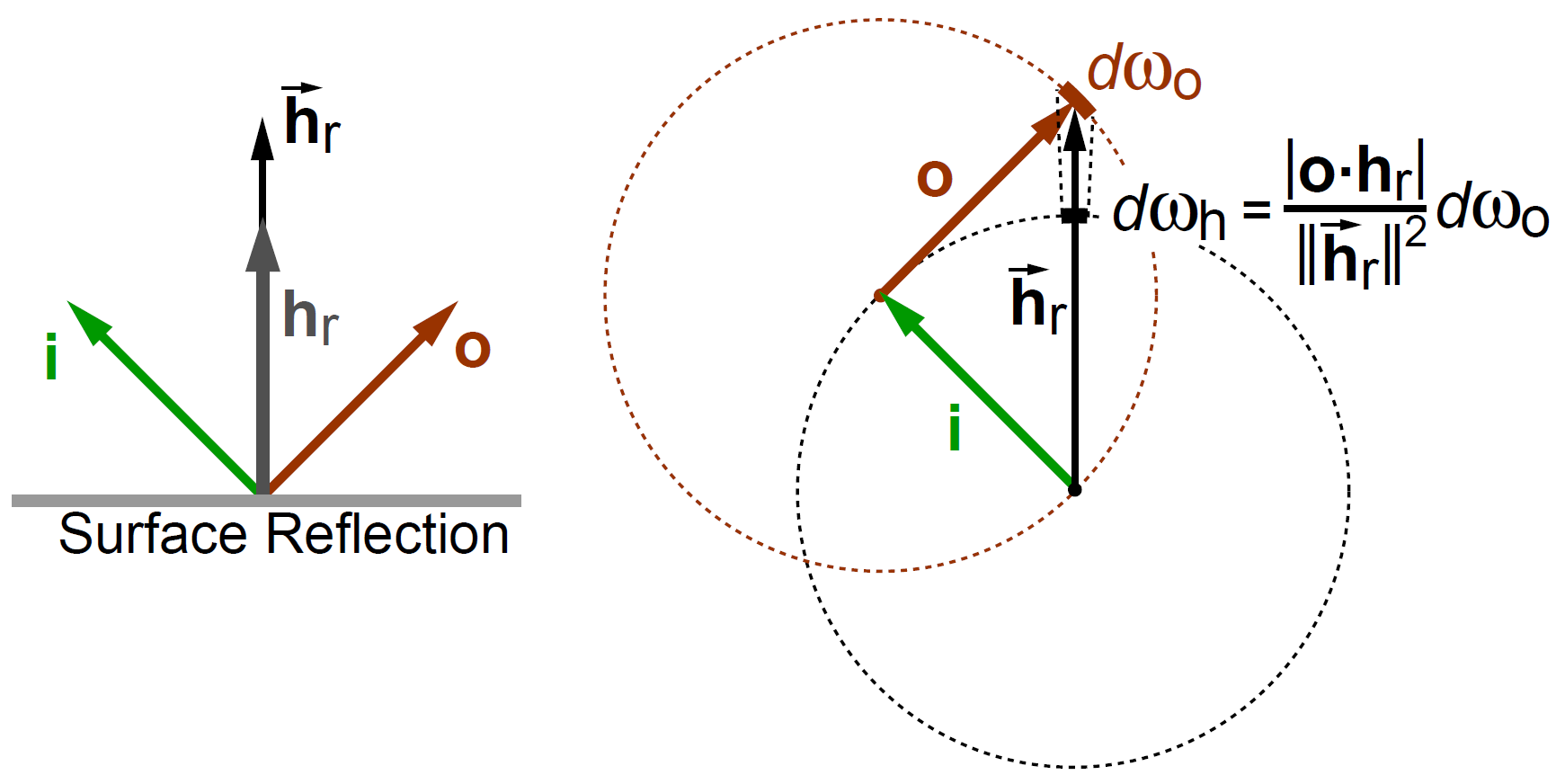
We can directly realize the relationship between $\mathrm{d}\omega_o$ and $\mathrm{d}\omega_h$:
\[|\frac{\mathrm{d}\omega_h}{\mathrm{d}\omega_o}| = \frac{|\omega_o \cdot \omega_h|}{||\vec{h}||^2} = \frac{|\omega_o \cdot \omega_h|}{(\omega_h\cdot\vec{h})^2} = \frac{|\omega_o \cdot \omega_h|}{(\omega_h\cdot(\omega_i+\omega_o))^2}=\frac{|\omega_o \cdot \omega_h|}{(2\omega_h\cdot\omega_o)^2} = \frac{1}{4|\omega_h\cdot\omega_o|}.\]Thus, we have:
\[f_m(\omega_m, \omega_i, \omega_o) = \frac{F(\omega_m, \omega_i)\delta_{\omega_m}(\omega_h)}{<\omega_i, \omega_m>} \frac{1}{4|\omega_h\cdot\omega_o|}.\]The microfacet BRDF
We are almost here! By substituting the microsurface brdf in the \eqref{eq: Statistical Microfacet BRDF}, we could get:
\[f_r(\omega_i, \omega_o) = \frac{1}{<\omega_i, \omega_g><\omega_o, \omega_g>} \int_{\Omega} G(\omega_m, \omega_i, \omega_o) \frac{F(\omega_m, \omega_i)\delta_{\omega_m}(\omega_h)}{<\omega_i, \omega_m>} \frac{1}{4|\omega_h\cdot\omega_o|} D(\omega_m) <\omega_m, \omega_o> <\omega_m, \omega_i> \mathrm{d} \omega_m .\]Since the delta term, we could solve this integral and get:
\[f_r(\omega_i, \omega_o) = \frac{1}{<\omega_i, \omega_g><\omega_o, \omega_g>} G(\omega_h, \omega_i,\omega_o) \frac{F(\omega_h, \omega_i)}{<\omega_i, \omega_h>} \frac{1}{4|\omega_h\cdot\omega_o|} D(\omega_h) <\omega_h, \omega_o> <\omega_h, \omega_i>.\]And now we get the microfacet BRDF:
\begin{equation} \label{eq: Microfacet BRDF} f_r(\omega_i, \omega_o) = \frac{F(\omega_h, \omega_i)G(\omega_h, \omega_i, \omega_o) D(\omega_h) }{4<\omega_i, \omega_g><\omega_o, \omega_g>}. \end{equation}